Solving little mysteries
This was originally written on 3 February 2019.
The next two fields in these old ULP files are titled, simply, “county” and “state.” These seem straightforward enough, but in fact getting these right is key to any project I want to do. Any hypotheses about where ULPs happened historically, and whether and how that changed over time, can only be tested if the geographic information is good. I need to lay some foundations for these to work.
Consider the relevant page from the code book:

Notice a few things here. No text is recorded in this file, remember; everything’s a code whose key is external to the file. Here, the codebook just points us to another codebook. Counties and states are recorded using a numerical code maintained by the General Services Administration’s Office of Finance. We have an example: Erie County, Ohio is encoded as 04334, i.e., Ohio is 34, and Erie County within Ohio is 043. To Google!
My first guess is that these are, at root, FIPS codes, part of the Federal Information Processing System. There are standardized FIPS-2 codes for the states, and FIPS-5 codes for the counties. (The first two digits of the latter are the state codes.) I’ve used these codes more times than I care to count, and have some Stata scripts that I use to encode such variables and give them nice value labels. I’m trying to do these things in R, though, and so I want to rebuild material like that.
A quick search of the General Service Administration’s site reveals that, yes, the Geographic Location Codes are based on the FIPS, and they have available for download an Excel file filled with cities and their relevant geographic codes:

The problem here is that I only need unique county codes. This file has unique city codes, which means it repeats many of the counties many times. It’s okay, though. This is why the Good Lord gave us Emacs.
This is not the place to sing the praises of Emacs. Suffice it to say that, if you scale no other learning curve in graduate school, you should just learn how to use Emacs. (This is just my opinion, but I am right.) Any number of bonkers tricks are possible with Emacs, but one of the ones I use most often is manipulation of structured text like this, through the use of regular-expression replacements and keyboard macros.
I wrote up a detailed example of how you might transform that Excel file into something like this using Emacs…

…but I deleted all of it, because it felt more like I was showing off than like I was imparting useful information. In point of fact, there are many, many good tutorials on using Emacs to be found online and indeed within Emacs itself. And, to be fair, a lot of people who have no fear of complicated text manipulation nonetheless despise it. (I’m looking at you, Vi users.) I think it’s the best thing for a lot of our work, but the larger point is that the power of a good text editor is not to be ignored.
And in any case, this post is supposed to be about solving little mysteries. Let’s get to that.
…In which everything goes wrong
Notice that that codebook page doesn’t specify which edition of the GSA’s geographic location codes it’s using. I figured that this file was created in the 1980s and covers 1963 through 1976, so I could use the 1976 edition of the codes. A quick check of the 1972 edition showed very little changes, and indeed the codings of the states and several prominent counties in the 1976 edition were ones that I recognize from the current editions. (There’s no state with the code 03 for example; we go from Alaska at 02 to Arizona at 04.) Based on these correspondences, I figured it would be safe to build county codes by transforming that Excel file from the GSA.
So, I did that:


Notice that the text names that I’m giving those counties–the labels that will appear once the factor variables are properly encoded–also have the two-letter state in them. This is important. Tons of states have Washington or Jefferson Counties (And Wyoming Counties! It’s a river in Pennsylvania, people!). If you don’t distinguish the state in the county names, the best-case scenario is that your function will fail because the factors are not uniquely identified. The worst-case scenario is that it doesn’t fail, and now you have multiple factor variables with the same label. This defeats the purpose of having labels.
So, I wrote up some long functions that would define factor variables for counties and states, with all the relevant codes and labels in them. I wrote these functions in a separate file, with the idea that I will re-use these a lot. That’s a good practice that’s almost as old as programming itself. Yet when I started tabulating the encoded data, I almost immediately saw problems.
I encoded the states, then started trying to check that the encoding worked. For example, I thought I’d make sure that counties were mapping uniquely to states. But that didn’t seem to be happening:
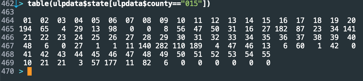
It appeared that the county designation 015 was spread across almost all states. This happened with others as well. For several minutes, I despaired, thinking that this project might be dead in the water. If the geographic location data wasn’t any good, there wasn’t much point continuing.
And then I calmed down
You might already have seen the problem here. When I defined the county-encoding function, I was careful to use the five-digit codes. The whole reason for doing so is because 015 shows up in many states. Yet when I tabulated the counts of that code across states, I just used the three-digit code, which of course repeats!
I mention all of this because this is a blog about doing a research project. And, for me at least, one unavoidable aspect of doing research is making mistakes and immediately thinking that
The data, and the whole project, might be trash from a nightmare realm
I am an idiot who doesn’t deserve to live, much less do research
The first is almost never true, and the second never is. Yet I find it distressingly easy to read too much into things like this and get discouraged. You might, too. So it’s worth mentioning.
That said, I still had a problem. When I tabulated the states, the counts looked all wrong:
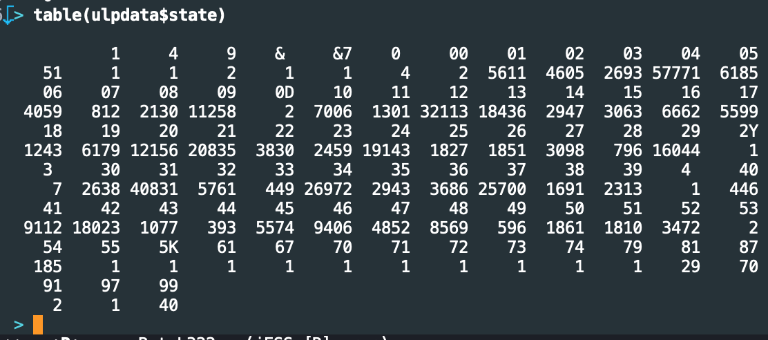
A thing about the output of R’s table() function: it lists values above then counts below, left to right. This is telling us for example that 1 record has the state recorded as &7, 5,611 have it recorded as 01, and so on. What I want you to focus on are the counts for 03 and 04. I mentioned above that the FIPS-2 doesn’t have a label for 03; so why are there 2,693 records with it? Furthermore, 04 is Arizona, while 06 is California. Yet here, 06 only has 4,059 records, while 04 has fully 57,771! That makes no sense.
Further inspection of these counts seemed to point to several large states being one or two positions off from where they should be. Notice the bunching around 37, which screams “New York”; but New York should be 36. But then 42, which encodes Pennsylvania, looks to be the right size…
Eventually, I surmised that the NLRB had kept using a much older edition of the GSA Geographic Locator Codes, long after revisions had come out. I surmised this because I’ve seen it in other federal datasets. The EEOC, for example, used 1987 SIC codes to track industries until the early 2000s, even though Commerce had nominally retired the SIC and switched to the NAICS codes in 1997. For the record, this isn’t a story of government sloth. Historical comparability across time periods is a big deal in datasets like these, and should be weighed carefully against updates to the coding scheme.
More Googling led me to a scanned copy of a 1969 edition of the GSA’s Geographical Location Codes, provided by the University of Michgan to someone. Before I go on, let’s just pause to admire this gem of a cover:

How old-school can you get? We’ve got magnetic tape; we’ve got punched cards; Hell, their example of a foreign-yet-familiar place is “Saigon, Viet-Nam!”
I love the smell of old documents in the morning. It smells like comprehension.
Inside was the key I needed:

Bingo. In the 1969 and earlier editions, California was coded 03, Pennsylvania was actually coded 37–but Texas was 42, which makes sense. Dig how Alaska was 50 and Hawai’i was 51. This strongly suggests that this edition included incremental changes from some point in the 1950s, before either became a state.
Let’s recap
This whole post is about the challenges of getting two simple variables coded. Nor are the codings themselves complicated. All I’m trying to do is apply “standardized” government labels to places. Yet we’ve seen code books referencing other code books, and we’ve seen how changes across time and place can complicate the application of even simple schemes.
We’ve also seen how important it can be to run multiple “sanity checks” on data as you build it. My encoding function ran without errors, after all, yet it produced semantic gibberish. Good exploratory data analysis involves repeatedly testing assertions about what should hold in the data, given your prior assumptions and what you’ve done to transform the data. Better to do this now than to get all the way to the analysis (or worse!) and have to backtrack dozens of steps.
Nor is any of this wasted time, even if you don’t find some confusing error that threatens to throw you into the slough of despair. Rooting around in your data, at this low level, is how you develop a sense of what’s in it. That intuition will be leveraged later on.